An impact-evaluation workflow
Source:vignettes/impact-evaluation-workflow.Rmd
impact-evaluation-workflow.RmdThis vignette walks from a study’s raw data to a baseline-equivalence
report, using the bundled (simulated) tutoring dataset.
library(baselinr)
data(tutoring)
head(tutoring)
#>   treat  pretest attendance  age female frpl ell posttest
#> 1     1 33.02273  0.9416614 10.2      1    0   1     49.8
#> 2     1 47.86310  0.9759478 10.0      1    0   1     53.0
#> 3     1 42.15184  1.0000000 10.3      0    0   0     49.2
#> 4     1 45.37557  0.9483293 10.7      1    0   0     57.4
#> 5     1 38.89146  0.9512494  9.4      0    1   0     49.3
#> 6     1 47.94922  0.9757792  9.4      0    0   1     43.8
tutoring is a simulated
quasi-experimental evaluation: 200 students who received a tutoring
program (treat = 1) and 200 who did not
(treat = 0), with baseline covariates and a post-program
posttest.
Step 1: assess baseline equivalence, before looking at the outcome
The credibility of any later effect estimate rests on whether the two
groups were comparable at baseline. We pass the
baseline covariates explicitly. We do
not include posttest, which is an outcome,
not a baseline covariate.
baseline_covs <- c("pretest", "attendance", "age", "female", "frpl", "ell")

equiv <- baseline_equivalence(tutoring, treatment = "treat",
                              covariates = baseline_covs)

knitr::kable(equiv, digits = 3)| covariate | type | n_treatment | n_comparison | mean_treatment | mean_comparison | sd_treatment | sd_comparison | effect_size | wwc_category |
|---|---|---|---|---|---|---|---|---|---|
| pretest | continuous | 200 | 200 | 52.150 | 50.099 | 9.824 | 10.993 | 0.196 | satisfied_with_adjustment |
| attendance | continuous | 200 | 200 | 0.927 | 0.918 | 0.053 | 0.049 | 0.186 | satisfied_with_adjustment |
| age | continuous | 200 | 200 | 10.044 | 10.034 | 0.508 | 0.504 | 0.020 | satisfied |
| female | binary | 200 | 200 | 0.530 | 0.525 | 0.500 | 0.501 | 0.012 | satisfied |
| frpl | binary | 200 | 200 | 0.555 | 0.445 | 0.498 | 0.498 | 0.268 | not_satisfied |
| ell | binary | 200 | 200 | 0.250 | 0.150 | 0.434 | 0.358 | 0.385 | not_satisfied |
baselinr automatically uses Hedges’ g for the continuous
covariates (pretest, attendance,
age) and the Cox index for the binary ones
(female, frpl, ell).
Step 2: read the categories
Each covariate falls into one of three What Works Clearinghouse categories:
equiv[, c("covariate", "effect_size", "wwc_category")]
#>    covariate effect_size              wwc_category
#> 1    pretest  0.19639834 satisfied_with_adjustment
#> 2 attendance  0.18641935 satisfied_with_adjustment
#> 3        age  0.01971405                 satisfied
#> 4     female  0.01215809                 satisfied
#> 5       frpl  0.26775010             not_satisfied
#> 6 ell 0.38544774 not_satisfied-
satisfied: the groups are equivalent on this covariate; nothing more to do. -
satisfied_with_adjustment: equivalence holds only if you statistically adjust for this covariate in the impact model. This is a commitment, not a pass: those covariates must appear in the model. -
not_satisfied: this covariate cannot establish equivalence even with adjustment. It’s a threat to the study’s credibility that you have to confront, not bury.
Step 3: visualise
love_plot(equiv)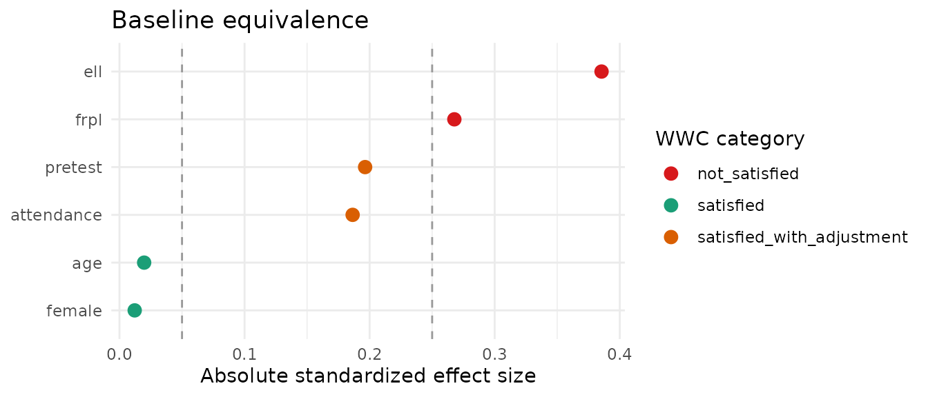
The dashed lines mark the 0.05 and 0.25 thresholds; points are coloured by category. The plot makes the at-risk covariates obvious at a glance.
Step 4: a report-ready table
For a written report or a Quarto/HTML document,
gt_baseline() returns a formatted gt
table:
gt_baseline(equiv)What this does and doesn’t tell you
baselinr reports the baseline equivalence picture. It
does not fit the impact model for you. The next steps
are yours: include the satisfied_with_adjustment covariates
in the model, and decide how to handle (or report the limitation of) any
not_satisfied covariate before you interpret the program’s
effect on posttest.