Your baseline table is doing more work than your p value
For a long time the baseline table was the part of a report I did last, fast, and a little resentfully. Throat clearing before the real analysis, was how I thought about it. Get it out of the way, get to the effect.
I had it exactly backwards about which part was the real analysis.
By the time you’re estimating a program effect, you’ve already placed the bet that matters: that the two groups were comparable to begin with. If they weren’t, you’re not measuring the program. You’re measuring the head start. No model downstream fixes that, and reviewers, funders, and the What Works Clearinghouse all know exactly where to look.
The question it’s actually answering
Plain version: before the program started, were these groups similar enough that I can pin later differences on the program instead of on who was in each group?
Notice what that is not. It is not “is the baseline difference statistically significant?” That’s the reflex, run a t test on the pretest, see p > .05, declare the groups fine, move on. But significance is the wrong tool here, for a reason that has nothing to do with the program. With a big sample, a trivial difference turns “significant.” With a small one, a real gap sails through as “not significant.” A p value is mostly telling you about your sample size. Equivalence is a question about size of the gap. Different question.
What the WWC asks for instead
For each covariate you report a standardized mean difference (Hedges’ g, which is Cohen’s d with a small sample correction), and you read it against two numbers:
| Hedges’ g (absolute value) | Category | What it commits you to |
|---|---|---|
≤ 0.05 |
Satisfied | Nothing. The groups are equivalent here. |
0.05–0.25 |
Satisfied with adjustment | Fine only if you adjust for this covariate in the impact model. |
> 0.25 |
Not satisfied | This one can’t establish equivalence, and adjustment won’t save it. |
The whole framework is those two numbers, 0.05 and 0.25, applied honestly. The arithmetic isn’t the hard part. Remembering what each category obligates you to do later is.
Doing it without a spreadsheet
Here it is on a simulated tutoring evaluation, 400 students, data I bundled into baselinr just for this. One call, whole table:
library(baselinr)
data(tutoring)

baseline_equivalence(
  tutoring, treatment = "treat",
  covariates = c("pretest", "attendance", "age", "female", "frpl", "ell")
)| Covariate | Type | Mean (T) | Mean (C) | Effect size | WWC category |
|---|---|---|---|---|---|
| pretest | continuous | 52.15 | 50.10 | 0.196 | satisfied_with_adjustment |
| attendance | continuous | 0.927 | 0.918 | 0.186 | satisfied_with_adjustment |
| age | continuous | 10.04 | 10.03 | 0.020 | satisfied |
| female | binary | 0.530 | 0.525 | 0.012 | satisfied |
| frpl | binary | 0.555 | 0.445 | 0.268 | not_satisfied |
| ell | binary | 0.250 | 0.150 | 0.385 | not_satisfied |
Continuous covariates get Hedges’ g; the binary ones get the Cox index, handled for you. And honestly the plot is where it clicks:
love_plot(baseline_equivalence(tutoring, "treat",
          covariates = c("pretest", "attendance", "age", "female", "frpl", "ell")))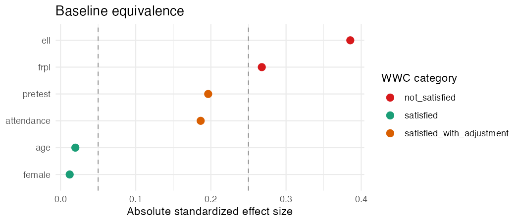
Age and sex are equivalent, nothing to do. Pretest and attendance sit in the middle band, so you can proceed but you owe the model an adjustment. And then poverty status and language status blow past 0.25, which means the groups differ on two things adjustment can’t fix. That last pair is something you’d want to know before you ever report an effect, not after a reviewer finds it.
The part that quietly leaks credibility
“Satisfied with adjustment” is not a passing grade. It’s a promise. It says: these groups are close enough, as long as I actually control for this covariate in the impact model. And it is genuinely common to see a baseline table that files a covariate under “satisfied with adjustment” and then an impact model that never adjusts for it. The table says one thing, the model does another, and a careful reader catches it instantly. If a covariate lands in the middle band, it has to show up in the model. Every time.
Treat the baseline table like the load bearing wall it is, not the trim you tack on at the end. Get it right and everything downstream has something solid to stand on. Get it wrong and your fanciest model is just measuring the head start.
I build baselinr, a small R package that produces these tables, and am developing a cohort course on credible evaluation and measurement in education. subscribe via RSS to follow along.